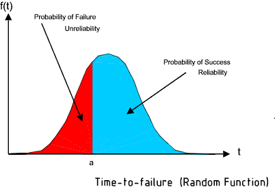
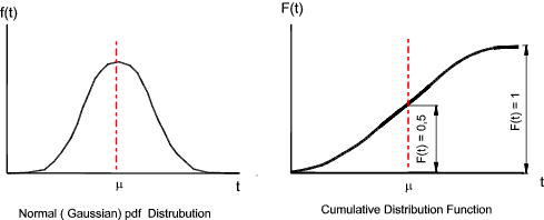
In determining the lifetime reliability of a population of components (bearings, seals, gears etc.) sample information is obtained from testing programmes and operational feedback on the failure history of components belonging to the population.  From the information obtained it is possible to produce a graph of the probability density function f(t).   This is a plot of the frequency at which components fail as a function of time divided by the whole population.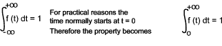

The pdf function has the property

Associated with the pdf is the Cumulative Density Function F(t).  This is simply a plot of the cumulative fraction of the failure population against time.  It is the integral of the f(t) against time (t).

The CDF has the properties

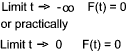
This effectively means that at time 0 no failures have occurred.

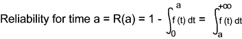
At infinity the whole population of components will have failed.

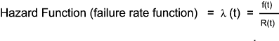
The reliability may be expressed that.. for time = a ( e.g 10 years ) there is a chance of the item surviving (not failing)... = 1 in 10 is likely to fail.

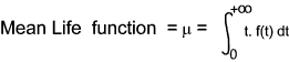
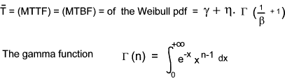
The hazard rate may be expressed as... the failure rate will be 2 x 10 ^-4 (failures /unit time) or 2 failures per 10 ⁴ time units

The mean life provides the average life to failure of components is also called the Mean Life Between Failures (MLBF) and the Mean Time to Failures (MTTF)

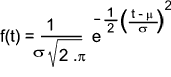
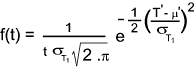
The MTTF /MTBF may be expressed as say 1,000 hours at which 50% of units have failed

The pdf curve can take many forms....Some of the different distributions are listed below

One curve representing purely random events is the normal (gaussian) curve.
This is shown below with the associated CDF.

The equation for the normal distribution is :

Both of these parameters are estimated from the data, i.e. the mean and standard deviation of the data.   From these parameters f(t) is fully defined enabling evaluation of f(t) from any value of t.

Note: The standard deviation is a measure of scatter of the information.    A small standard deviation is a thinner higher bell and a large standard deviation is a wider flatter bell.

Normal Distributions are appropriate in the following conditions

The lognormal distribution is commonly used for general reliability analysis, cycles to failure in fatigue and material strengths and loading.

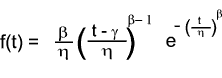
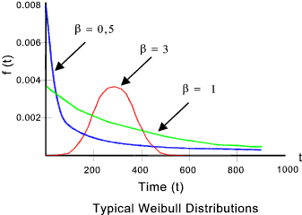
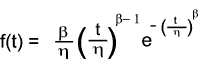
The data follows the lognormal distribution when the natural logarithms of the times-to-failure are normally distributed.

• σ_T1 = Standard Deviations of the natural logarithm of times-to-failure
• μ' = Mean of the natural logarithm of times-to-failure

The Weibull distribution is a general-purpose reliability distribution used to model material strength, times-to-failure of electronic and mechanical components, equipment, or systems.   In its most general case, the three-parameter Weibull pdf is defined by:

with three parameters, where :

If the location parameter γ is assumed to be zero then the distribution is known as the two-parameter Weibull distribution...

The β = shape parameter gives indications on the prevalent failure modes.

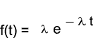
The exponential distribution is a commonly used distribution in reliability engineering.   Mathematically, it is a fairly simple distribution, which sometimes leads to its use in inappropriate situations.   This distribution is used to model the behavior of units that have a constant failure rate.

An exponential distribution can easily be described as follows...
If a thousand items have a constant failure rate of 10% per month.  After the first month 100 items have failed (0.1 x 1000) leaving 900 items.  After the second month 90 items will have failed (0.1 x 900) leaving 810 items...  After 12 months 31 items will fail leaving 282 items.

The mean time to failure of this distribution is

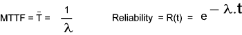
If the location parameter γ is assumed to be zero then the distribution is called the one parameter exponential distribution.

The mean time to failure and the reliability of this distribution is