Introduction
Note: The notes below are generally provided without proof. For more detailed notes
refer to the links below:
In an experiment more than one variable may be recorded e.g. The strength
of a steel specimen (say variable X) and the % elongation (say variable Y). It is possible to plot the resulting values
from a number of these experiments on as points on an X Y plane. Each experiment results in a value X= x and a value Y = y.
Considering the case of c1 < X ≤ d1 , c2 < Y ≤ d2 which includes
all of the outcomes that lie in the enclosing rectangle.
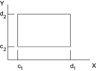
The probability of this case is
P (c1 < X ≤ d1 , c2 < Y ≤ d2 )
The two dimensional probability distribution is expressed as
F(x,y) = P ( X ≤ x , Y ≤ y )
The probability distribution function expresses the distribution uniquely because
P (c1 < X ≤ d1 , c2 < Y ≤ d2 ) = F (d 1 d 2) - F (c 1 d 2) - F(d 1 c 2) + F(c 1 c 2)
Symbols
P(x,y) = probability function for two values. (values between 0 and 1)
F(x,y) = probability distribution function for two values.
f(x,y) = probability density function for two values.
Φ (x) = Probability distribution function.(Standardised probability )
μ = mean
σ 2 = variance
σ = Standard deviation
ρ = correlation coefficient
|
Discrete Functions
Bivariate probability distributions.
The variables and functions are discrete if ( X , Y ) can assume only countable (as opposed to
measurably) many pairs of values of ( x , y ) and the corresponding probabilities are positive.
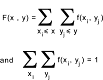
The probability density function f(x,y) = p i j when x = x i and y = y j
and f(x,y) = 0 otherwise.
The associated probability distribution functions are as follows .
Marginal probability distributions.
In the case of a discrete random variable (X,Y) with a probability of f(x,y). There needs to be considered the question
of what is the probability P(X = x, Y = any value) that is, what is the probability
of X= x while Y is arbitrary -it can assume any value.
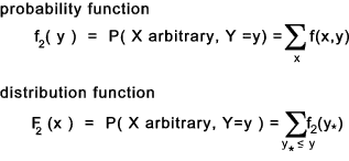
For this situation the probability is a function of
x = f1 (x) such that all the values of f(x,y) for that x which are not 0 are summed

This is the probability distribution of a single random variable
which is called the marginal distribution
of X with respect to the given two dimensional distribution. The distribution ...

Where x* is the transformed x as defined above.
The probability functions and distribution functions of the marginal distribution of Y with respect to the the joint distribution is similar.
Continuous Functions
Bivariate probability distributions.
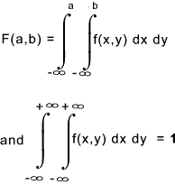
A continuous distribution function of a pair of variable can be represented by the double integral
Marginal probability distributions.
Considering the case of the continuous random variable (X,Y) with probability density function f(x,y) for the probability that X =any value up to x whilst Y can be any value, that is ,Y is arbitrary

This has a probability

Setting the probability density function of x

This is called the marginal distribution
of X with respect to the given two dimensional distribution
The relevant distribution function may be written

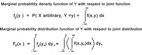
Considering the case of the continuous random variable (X,Y) with
probability density function f(x,y) for the probability that Y =any value up to y whilst X can be any
value, that is ,X is arbitrary. similar equations result
Bivariate Normal distribution
An important continuous distribution is the bivariate normal distribution. This
function is express mathematically by.

A typical distribution based is shown in the diagram below. This resembles a
hill on a flat plain
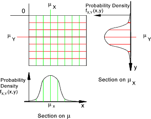
Both variables have their ownparameters for mean and variance.
μX , μY , σ 2X and σ 2Y.
An additional parameter ρ is required which is called the correlation coefficient . This summerises the
degree of association between X and Y.
Independent variables
The distribution function of truly independent variables (discrete or continuous) has the properties .
f (x 1, x 2..x n) = f 1(x 1) .f 2(x 2)....fn(xn)
F (x 1, x 2..x n) = F 1(x 1) .F 2(x 2)....Fn(xn)
Consider n independent normal random variables X1, X2...Xn
with means
μ 1, μ 1...μ n, and variances
σ 1, σ 1...σ n the random variable X exists with properties..
X = X1 + X2 ...+ Xn
mean = μ = μ 1 + μ 2...+ μ n
variance = σ 2 = σ 21 + σ 22....+σ n 2
Example 1:
Consider three purses, one containing 10-5p coins and one containing 10-10p coins
and one containing 10-20p coins .
The masses of the three coins are assigned the variables X1, X2
and X3.
The mean values of the relevant masses are say
μ1= 3,25 g, μ2= 6,5 g
and μ3 = 5g respectively.
The variances of
the relevant masses are say σ 21= 0,20 g 2, σ 22= 0,25 g 2 and σ 23= 0,15 g 2
Repeatedly taking one coin from each purse results in collections of three coins to the value of 35p.
The combined weight of the three coins is X.
X has a mean mass of μ =(3,25 + 6,5 + 5 = 12,75 g) and a variance of μ =(0,20 + 0,25 + 0,15 = 0,6 g 2)
Example 2:
In the UK the average weight of and adult is say 60kgf with a standard
deviation of 6 kgf. What is the probability that the combination of 10 people in a lift
will be less than the design weight of 650 kgf.
The problem is simply the combination of 10
normal distribution each with a mean
of 60 kg and a standard deviation of 6 kg.
The mean value of the laden lift occupants = 10 ,60 = 600 kgf.
The standard deviation of the laden lift occupants = 
Now z = x - μ ) / σ = (650-600) / 18.97 = 2,63
Φ(2,63) = 0,9957 = 99.6% .this is the probability that the weight will
be less than 650 kg.
|