Probability distributions for continuous random variables differs from discrete distributions variables in the following important aspects:

1) A variable can take on any, of an infinite number of values within the range

2) The probability of any specific value is zero.e.g The probability 50mm ± 0 is zero.

3) Probabilities are expressed in terms of an area under a curve of the continuous probability distribution.

In engineering as in most other disciplines it is useful to determine patterns which indicate the probability of variables and events e.g in the mass production of 50mm diameter shaft on a lathe... what is the probability of the shafts being within the acceptable tolerance limits .  Probability curves show the variable on the x axis and the probability f(x) of the variable on the y axis.   The total area under the curve represents the probability of all possible events and equals 1

There are a number of continuous probability distributions which are used for different probability conditions.  The most widely used is the normal probability distribution also called the Gaussian probability distribution.  This represents the probability conditions most representative of events that occur in the natural world subject to countless variables.

The normal probability distribution has the following characteristics

1) The graphed distribution curve is bell shaped and is symmetrical about the mean value

2) The mean, median, and mode are the same.

3) The distribution is defined by the mean span>μ and the standard deviation σ

4) The distribution extends from negative infinity to positive infinity

The mean value of a distribution is denoted by μ and is defined by

The variance of a continuous distribution σ² and is defined by

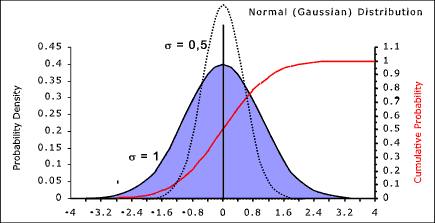
f(x) is the probability function of the random variable X under consideration.   The defintion of f(x) for a normal distribution is provided below.

The probability that is a single trial the variable will assume a value ≤ x is called the distribution function

A typical normal probability curve drawn with a mean value μ= 0 and a variance σ ² = 1 is shown above.

For this case the probability that is a single trial the variable will assume a value ≤ x becomes

(This function is plotted on the webpage Standardised Normal Distribution Table:
The values for this table have been obtained using the standard functions available on Microsoft Excel.)

This corresponds to a probability function

Note:
If v = (t - μ ) / σ then dv / dt = 1 / σ . Therefore dt = dv σ
Now considering the equation above for F(x) and letting v = (t - μ ) / σ

This is clearly = Φ(z) where z = (x - μ ) / σ
that is

It is very easy to obtain the probability that a variable x meets the criteria ( a < x < b ) using the tabled values by using the relationship.

Standardised Normal Distribution Table

The webpage linked provides values for Φ(z) for the range z = 0 to 4,19 .
It can be used for values -4,19 to 4,19 by using the relationship Φ(-z) = 1 - Φ(z)

a) Determining the probability of value is between a = μ - σand setting b = μ + σ using the tables result in simply looking up the difference in values Φ (1) - Φ (-1) = 0.841345 - (1- 0.841345) = 0.68269

b) Determining the probability of value is between a = μ - 2σand setting b = μ + 2σ using the tables result in simply looking up the difference in values Φ (2) - Φ (-2) = 0.97725 - (1- 0.97725) = 0.9545

c) Determining the probability of value is between a = μ - 3σand setting b = μ + 3σ using the tables result in simply looking up the difference in values Φ (2) - Φ (-2) = 0.0.99865 - (1- 0.0.99865) = 0.9973

The above simple calculations show that if a population conforms to a normal probability distribution
About 2/3 of the population values lie within the range μ - σ and μ + σ
About of the population values lie within the range μ - 2σ and μ + 2σ
About 99% of the population values lie within the range μ - 3σ and μ + 3σ

The relationship applies to all normal distribution.

Determine the probability P( x ≤ 10,5 ) for a x is normal with a mean (μ) = 10 and a standard deviation (σ ) = 2.

There is a 60% probability of x being less than or equal to 10,5

The values of p in the binomial distribution and μ and σ are the called the parameters of the distributions and it is frequently necessary to obtain values for these parameters from a given sample of a population.   It is often sufficient to obtain an estimate of μ   ( x_m is approximately equal to μ ) using the equation ref.Sample Variables

and it is possible to obtain an estimate of the variance ( as s_x is approximately = to σ using the equation ref.Sample Variables

In the case of the binomial distribution the p is easily estimated as being approximately

p = approximately x_m / n

For normal probability distributions good evaluations of the parameters can be obtained using normal probability paper.   This is graph paper with the lines arranged such that a normal probability distribution is plotted as a straight line.

Normal probability paper can be downloaded free from    Weibull Probability Plotting Papers